Nice to meet you! I'm Shin, a rising sophomore at the Massachusetts Institute of Technology studying mathematics and computer science. I'm very grateful to have been given the opportunity to spend an amazing six weeks at the LINE Tokyo office to work on an exciting internship project: "Improving reliability and consistency in metric anomaly detection".
Not only was it one of my first few work experiences in the tech industry, it was also my first time in Japan. There were so many learning experiences and eye-opening encounters that made up this unforgettable journey.
Let me take some time to walk you through my six weeks here.
Motivation
Anomaly detection has always been a crucial subject of interest. Anomalies occur for reasons that make them anomalies; they are unexpected, and usually they signify something perhaps wrong with the existing system or something that we do not fully understand, prompting further investigation into their root cause. For example, a spike in the number of API calls could be due to an attack from API abusers. Detecting this would allow engineers to enhance the system, guarding against these attacks that can impact the whole platform ecosystem.
Yet, many challenges lie in the accurate detection of these anomalies amidst the inherent noise present in the metrics data. For instance, take a look at the following plot (just one example of the many metrics we are monitoring).
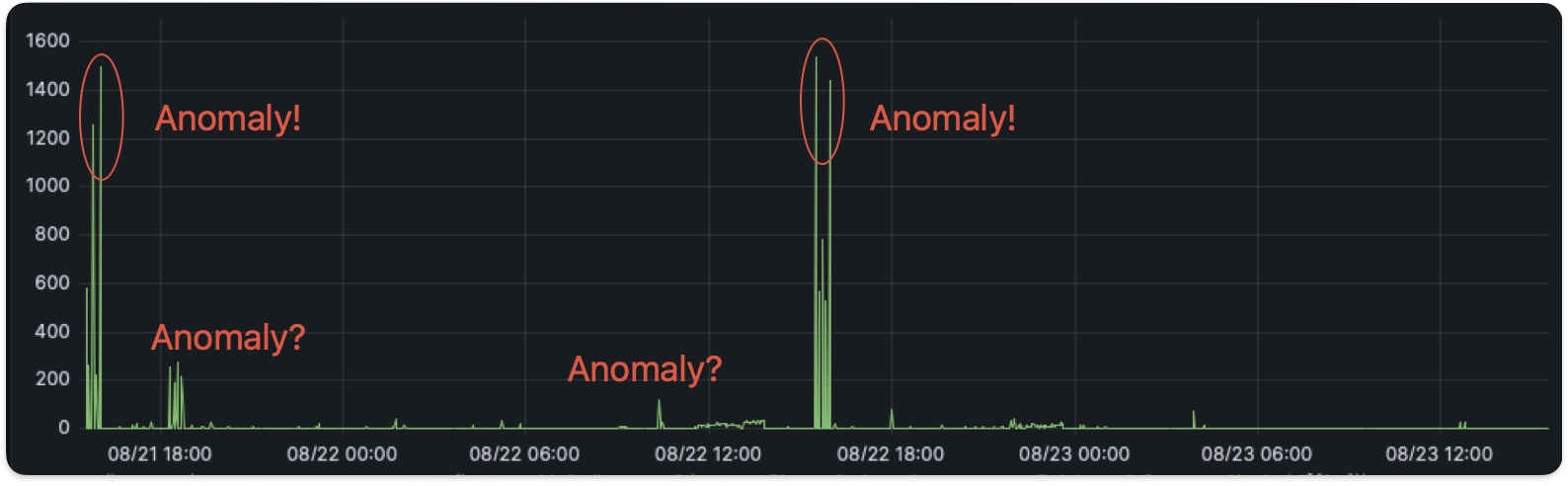
With the little and big spikes popping up here and there, how large would a spike need to be to be considered an anomaly? If there was an anomaly and we didn't detect it (a false negative), then some flaws within the system would have escaped our radar. Whereas, if there was no anomaly when the algorithm said yes (a false positive), then this would take up precious developer time to investigate something unfruitful.
The purpose of this project will be to build on existing models and finding improvements to create a consistent and reliable anomaly detection algorithm, minimizing the occurrences of false positives and false negatives.
Existing models
Static thresholds
One of the most basic models to start off with will be to set a fixed threshold for metric values and report an anomaly if the current value exceeds this threshold. With such a simple alert system, we can already capture much of what makes an anomaly and we can detect many anomalies quite reliably.
However, there exists a significant number of drawbacks that we should be aware of. The precise value of the threshold is currently quite arbitrary and depends on the values of the metric itself. When the metric value moves up and down, a fixed static threshold will be insufficient.
Look at the following example:
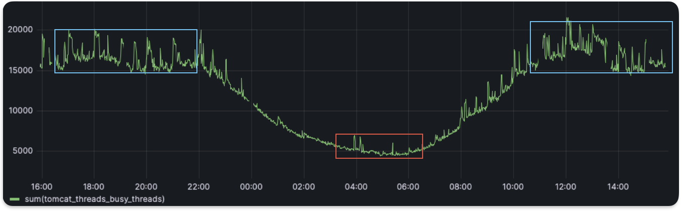
In this case, when the metric value is below 5000 (red region) there can still be anomalies due to the small spikes (of size ~1000). However, if we set a threshold to 1000, that would not work in the blue region where due to the noise in the metric value itself, values easily exceed 1000. Also, some metrics are inherently noisier than others, and we cannot use the same static value as a one-size-fits-all threshold. To resolve this, we turn to a standard approach of calculating the Z-score.
Z-score
A commonly used proxy for evaluating the presence of anomalies is the Z-score. Sometimes also referred to as the signal-to-noise ratio, this score captures, as its name suggests, the ratio of the signal that is the big spikes, to the inherent noise that is the random fluctuations in the data.
Computing the signal is quite straightforward: we take the difference between the current value and the mean value. However, how do we measure noise? Canonically, we measure this with the standard deviation. This allows us to write the Z-score as 𝑧=𝑥−𝜇𝜎 where
Making use of the Z-score allows us to solve some problems that we have faced previously. Computing the standard deviation for different types of metrics allows us to determine different thresholds to set for different metrics. Additionally, establishing a lookback time window to calculate the mean and standard deviation lets us have a dynamic threshold. This means during periods of high noise, the threshold is larger, and during quieter times, even a smaller spike can be treated as an anomaly.
Assuming that the metric values are distributed according to a normal distribution, we can place some mathematical guarantees on the probability of false positives. For example, we can show that with a threshold of
So this is all good. Are we done? Nope. Firstly, the assumption of a normal distribution is not exactly accurate, particularly when anomalies occur they do so more obviously, with an extremely large value. So we should expect not the continuous tail of a normal distribution but a cluster of points towards the far right (more on this later)! The distribution is also unlikely to be symmetric since we are more likely to see spikes upwards rather than downwards. Secondly, the computation time required for obtaining mean and standard deviation is rather costly. Think over a 1-hour window with update intervals of 1 second, we need 3600 data points per second to update mean and standard deviation! Summing that over all the metrics we have to monitor, that is an absurd amount of data!
Improvements
We have seen the potential advantages and drawbacks of existing models, and hereon the remainder of the blog will be dedicated to finding improvements in terms of accuracy and computation time.
A good reference would be the exponential moving average. Again, if
- It's just a single value: if metrics are updated once every second, a classic moving average window for 1 hour would result in a calculation involving 3600 data points each time step, whereas computations using this exponential moving average only does arithmetic involving a single value each time step
- It implicitly captures all the previous data points: once a metric value is seen, it is "remembered" forever! However, this might also be bad since we want to choose an
𝛼 small enough such that we don't just look at the data point right before, but also large enough such that points too far back aren't given too much weight - It accurately gives more weight to the more recent data points and lower weight to previous ones: the value of
𝑥 one time step ago will contribute only1−𝛼 that of the current value of𝑥 , and the value two time steps ago will incur a factor of(1−𝛼)2 .
So now we have a good proxy for a benchmark of "mean". And fortunately, there's also a formula for exponentially weighted standard deviation!
𝜎(𝑡)←(1−𝛼)(𝜎(𝑡−Δ𝑡)+𝛼(𝑥(𝑡)−𝜇(𝑡−Δ𝑡))2)
We can set the threshold
𝑐(𝑡)=𝑐0(𝑡)(1+𝛽𝑒−𝛾𝜏)
where
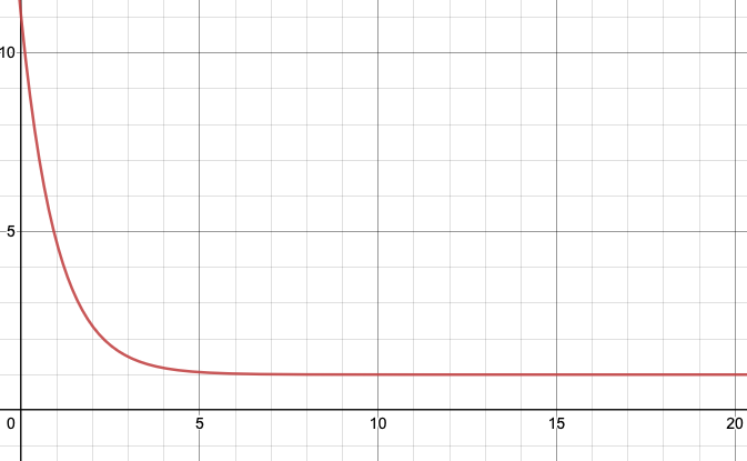
The 𝑥-axis is the time since the previous alert and 𝑦-axis is the threshold.
Architecture outline
To deploy the above strategy, several setup steps need to be taken to store the intermediate calculations. Much of the architecture involved concepts I wasn't initially familiar with. However, I'm grateful for the help I received from everyone, which allowed me to understand how to piece everything together.
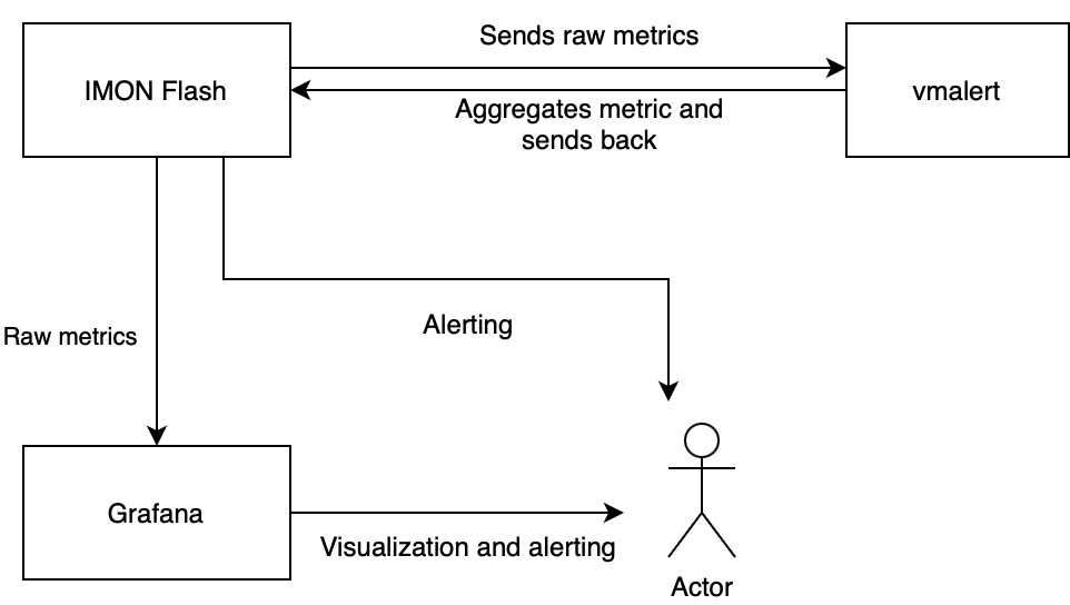
The majority of the data was stored on IMON Flash (LINE's internal database) as a Prometheus time series, which basically records everything we care about all of the metrics related to LINE's service. That's a lot of data! Grafana was used mainly as a visualization platform that allowed me to generate many of the graphs shown in this blog to gain an intuition for the different metrics themselves. The querying and recording infrastructure, vmalert, was only very recently integrated into our monitoring system, providing the perfect platform to allow dynamic update of values like
Many (in fact, probably all) of the terms used above were things unknown to me at the start of the internship. It took several days or even weeks to get a feel for each bit of the machine, including learning how to use minikube, setting up my own Kubernetes cluster for local deployment, installing a Helm chart, and thinking of better ways to use if-else statements while writing PromQL queries.
I learnt many things along the way, even those that weren't directly related to the diagram above, and eventually managed to implement all the ideas I had above into actual deployment.
Sample implementation
The following entries into the YAML file allowed implementation of the above strategy on a sample metric, tomcat_threads_busy_threads with parameter values
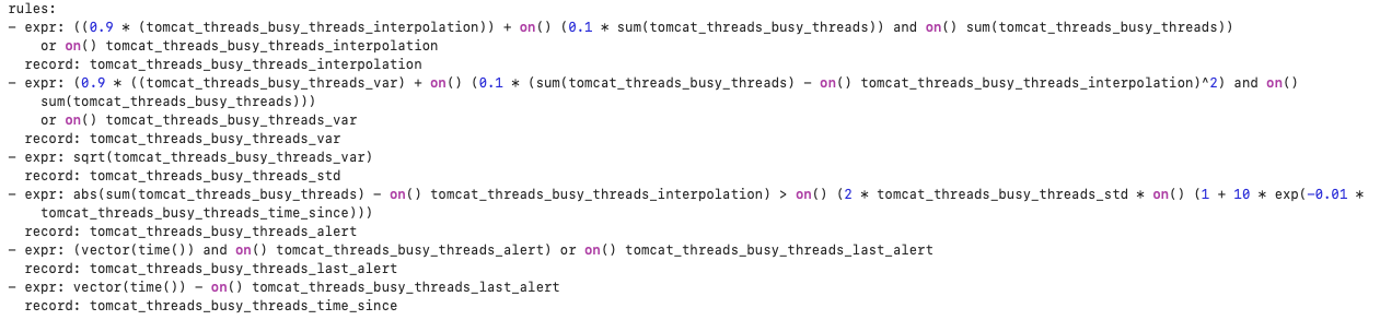
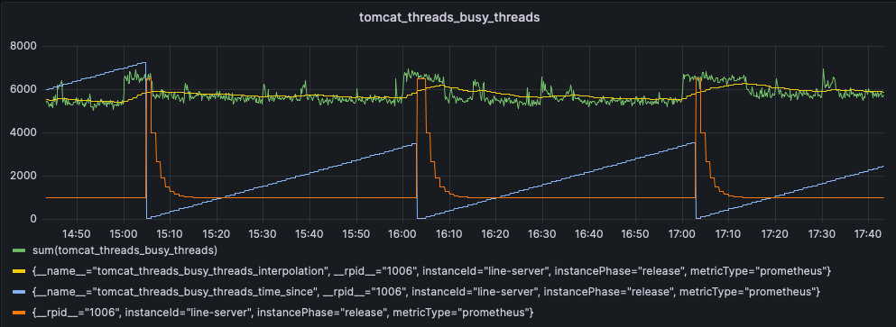
Yellow: exponential moving average
Orange: difference threshold 𝑐(𝑡)
Blue: time since previous anomaly
What we can see here is that there seems to be a noticeable jump in the metric value near each hourly interval. Our algorithm picks that up as the time from the previous alert drops to zero at the corresponding points of spikes in the graph. Such a regular occurrence might be due to LINE bots activated on exact hours, unlikely to be API abusers, but it's something interesting nonetheless! Again, whether or not we consider this to be an anomaly depends on our definition of what an anomaly is, but this works as a proof-of-concept for our proposed algorithm.
Improving on Z-score - obtaining the empirical distribution
We have spent much of the time developing and implementing a dynamic algorithm that nicely captures the ideas of mean and standard deviation, but there's still one problem left untouched. Classifying anomalies based on the standard deviations makes some assumptions on the underlying distribution from which the metric values at each time step is drawn from, specifically a normal distribution. Deviations from this ideal distribution will lead to inaccurate guarantees for how well our algorithm works.
This section will be dedicated to investigating the statistical distribution of the metric itself and constructing the necessary thresholds that gives us the mathematical guarantees to how well our algorithm would perform.
We divide the day into 24 hour bins and group the metrics according to their hours. What we do is obtain the empirical distribution for the raw metric values every hour. This way, we don't have to assume the existence of a normal distribution.
It might be of some interest to technically sidetrack a little here. Previously, we were concerned about the real-time computational cost of the algorithm as the anomaly detection system runs live. If the code took too long to execute, a timeout occurs and the algorithm is aborted. However, we can avoid this by using the IMON Flash API. We make repeated queries to the database that are just below the timeout threshold. This way, we can gather as much data as we need to get a precise distribution. In doing this, we may be slightly misusing our internal API for data analysis.
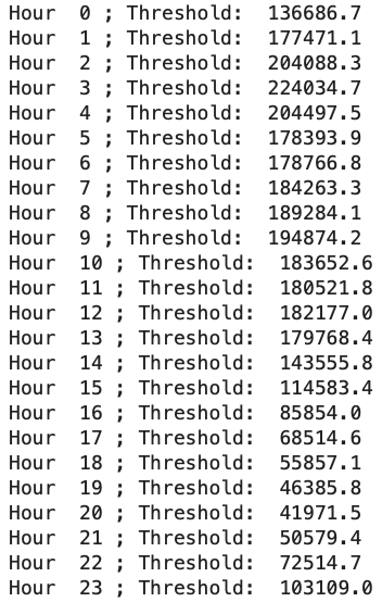
Returning to the main topic, for each hour, we identify, for example, the 95th percentile and set that as our threshold value. Below is a sample histogram for the raw metric values (not the Z-score) within hour 3 (from GMT 0300-0400). It also shows the 95th percentiles for all hours of the day, with data collected over 28 days. In this case, we set the threshold to around 224,000. This means that about 5% of the observed raw metric values are above 224,000. If the histogram represents the distribution of metric values without anomalies, and we observe a metric value above 224,000, the chance of it not being an anomaly is less than 5%.
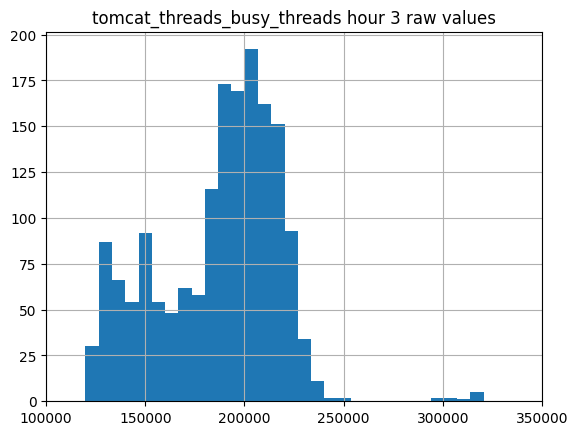
We can also observe a few things from these results. First, this distribution appears to be bimodal. The mean value might vary depending on the day of the week due to different behaviors of LINE users and bots on weekdays versus weekends. Second, our 95th percentile might not work too well here as we could catch some false positives with values around 230,000. Finally, there seems to be a small but distinct cluster of points with high values, around 300,000 on the right. This could suggest a cluster of anomalies captured in this histogram. We could use a clustering algorithm like k-means to distinguish the various peaks and identify anomalies.
We performed k-means (with
There are of course, some limitations to this implementation. Clustering might not always work, especially in cases where the cluster of anomalies aren't too distinct. We divided the day arbitrarily into hourly bins while our previous algorithm was an exponential moving average without such notion of an "hour". It would be great to combine what we have done in the previous two sections for something that works nicely in practice!
Future work
Much of the work done here is closer to proof-of-concepts and prototypes rather than complete products, so much work remains to be done. Just to name a few:
- Extending the above strategies to automate for all metrics in IMON Flash
- Integrating the 24-hour bin classification with the dynamic threshold
- Tuning alerting parameters according to feedback on performance, such as accuracy of detection on false positives and false negatives
- Pin-pointing the problematic server instead of a full-on aggregate detection (which might also miss server specific anomalies)
A lot of potential development lies within the infrastructure that has already been set up, but many other models can be explored, such as:
- Binary searching for the problematic server, using a majority voting algorithm
- Curve fitting daily trends instead of hourly-bins
- Sliding window max, min, and median calculations can be done in linear time using more advanced data structures, but might take a bit more effort to implement on vmalert
- Supervised machine-learning models to determine the probabilities of a metric value being an anomaly
Reflections!
Thanks for reading this far, I hope the statistics and engineering mentioned in this blog was an interesting read!
There were ups and downs during this internship, times where things were stagnant for a while, times where everything moved so fast, days where I didn't know what I was doing, and days where everything felt like they were falling in place. I'm very grateful to the Messaging Platform Engineering 2 (MPE2) team for welcoming me on board, members of LINE Platform Development Center 1 (LPDC1) who provided the technical support, people in the office who made the work day so much livelier (and healthier, by taking the stairs from B3 to 31F), and to all of LINE for giving me this learning opportunity in Japan.
I got to taste the best cuisine in the world, enjoy some of the most scenic views that seemed almost otherworldly, meet the most interesting collection of individuals with diverse experiences and backgrounds, and grow so much as a student and an engineer in the process. Now that the six weeks are drawing to a close, it feels like a sweet and surreal dream that I can only wish lasted a bit longer. For now, I will take whatever I have gained here back with me to school for another year, and hope that our paths may cross again someday.
Till next time,
Shin


")