
Hello everyone, I'm Dekai Wah, currently an intern at LINE's Game Security Department. In our department, we work on different facets of securing games from cheating behavior. These could range from obfuscating code to analysis of suspicious behavior on our game servers. In this project, my teammate Yoshiki Kusama and I analyzed the game data retrieved from our game servers and just as mentioned in an earlier article, find new ways to or better methods to detect game cheating behavior. This is a short introduction on cross-validation, parameter tuning, and evaluation. If you are interested in applied machine learning (ML) from a point of view of someone who has minimal knowledge in the subject, please feel free to read on. While we are certainly no experts in ML, the whole process from zero was interesting and insightful, from the setting up of the model, to the tuning.
The problem statement
At the first mention of "in-game cheating," it is impossible to pinpoint a particular marker for cheating behavior. Some tell-tale signs of cheating behavior are
- Having anomalously high game scores for each level
- Abnormal in-game purchasing behavior
- Clearing levels in an unrealistically short time
- Owning unrealistically high levels of in-game currency without purchasing records
For example, if a player obtains game currency or has a game score record which are both abnormally high for their in-game level, there is a possibility of a memory cheat or a packet editing cheat. Hence, the warning signs of such an abuser is the sudden and drastic increase in currency, merchandise or score records. These facts could be used as a factor in differentiating an abuser from a player who is not. The list is not exhaustive, and it becomes hard to combine all these factors right from the start.
Currently, as LINE GAME starts to get more and more popular, it becomes difficult to rely on human effort alone in manually banning suspicious users with the active user count increasing rapidly. While it is still very manageable now, it may not be the most scalable solution in the long run. Hence, our goal is to be able to combine all these signs of cheating behavior into a ML model, so that large-scale banning can take place without any need of intervention. To have some insight into the feasibility of using ML, we have attempted to construct a model based on in-game currency volumes.
The idea
While I believe most of our readers have some knowledge of what ML is (since it is a trending buzzword), here is an overview for those who are not familiar with the term. ML is an application of Artificial Intelligence - should users pass in a set of data, the machine will learn and improve in its detection of patterns within the set of data with each iteration. As the name goes, the machine "learns" the criteria or sorting method, and this can fulfill many use cases. In our case, the game data was used as the main dataset for the machine to derive insights from. We hoped that the machine could learn the difference between a non-abuser, and an abuser, so that it could detect abusers automatically and quickly. Then, it would be a good idea to bring in the idea of supervised learning at this point.
Supervised learning is the method in which machines process data with labels in it. Labels are categories attached to each datapoint, that could tell the machine which group or type that datapoint belonged to. In our case, our extracted data from the Game server has abusers (who have been banned, or have abnormally high amounts of game currency), and non-abusers. By "labeling," we really mean putting a category for each user, either 0 or 1, where 0 stood for a perfectly normal user whom we deemed to be a regular game user, and 1 stood for a user who showed evidence of cheating. Hence, by feeding these labelled data sets (where we explicitly tell the machine whether each user is an abuser or not), it serves as what others call "training data." We train the machine on this dataset, in hopes that it can provide us answers to whether the new, unknown users are abusers or not. As an analogy, it is not unlike taking a mock examination paper with given answer keys, before taking an actual examination. The infographic below gives a good idea on what we are aiming for.

Hence, our hopes are that the machine could detect abusers with high accuracy based on previous labeling already done.
The data
In our game database, we currently have 26 sets of variables that can be publicly mentioned. For better visibility, we split the available data into types. Without going into too much detail, there are 4 variables which account for game currency data, and we will label them as 1coin, 2coin, 3coin, and 4coin. We have also replaced all game-defining play information with a generic gamefeature name, to protect the game's identity. Game features are also simplified into gamefeature1 through gamefeature4.
- User Information (pertaining to game currency, game experience and levels):
lv,exp,allcoin,SHC,2coin,pheart,bheart,1coin,userruby - Play Information (pertaining to game scores or game achievements):
GF1,gamefeature1,gamefeature2,skillcnt,gamefeature3,AC,avgcoing,gamefeature4,playcnt - Rank Information (pertaining to game performance):
rank1cnt,rank2cnt,rank3cnt - login Information (pertaining to login counts):
logincnt,cntlogincnt,maxlogincnt - Other:
tutorialflg,invcnt
Hence, there are roughly 5 big groups of information that we can use in our modelling for this situation. In our first testing scenario, we wanted to look for a model that could generally pick up on abnormally high values of game currencies. For this reason, in our first testing model, not only were banned users labelled as abusers, users with abnormally high values of game currencies (variables: 1 coin above 9,999,999 & 2 coin above 100,000,000) were labelled as such as well.
However, in fear of overfitting, these coin values used to label the data (1coin & 2coin) were not considered in the training of the model later. This is because, while we would get a near perfect accuracy, we would not be able to get a good view on other cheating behaviors as well. Hence, in our initial labeling of data, our data sample had the following breakdown:
| 0 (Non-abuser) | 1 (Abuser) |
|---|---|
| 94,833 | 15,165 |
With over 100,000 datapoints, this seemed to be a good amount for the model to learn adequately, while maintaining speed of the ML algorithm. Even though the data seems to be slightly imbalanced, we can deal with this later.
The model
We needed a robust model which could be accurate and flexible in purpose. Especially when in the dataset, there would be a lot of data that do not follow a set pattern (such as users with 0 scores and level 1, or abnormally low scores due to inactivity during playtime), we also needed to look at a model which is not highly affected by noise. In addition, it is also unknown to what extent each of the 26 data features are relevant to the abuser classification and this makes noise resistance one of the most important choice factors. The labeling of output (Abuser vs Non-abuser) seems to be the central problem, and hence, this can be thought of as a classification problem. Hence, we arrive at the conclusion that the random forest model could be a good model as a test-start for this project. The whole classification tree can be thought of to work out like this:

This is a rather robust model as each datapoint (user) is classified using a series of decision trees. The ML model would split the categories further and further down within each decision tree. For each decision tree, a datapoint's final classification goes towards a vote. Hence, we say that the datapoint is classified (abuser or non-abuser) using each tree, and then the series of results compared (which numbers more, abuser or non-abuser) to decide if the datapoint is an abuser or not. Hence, the numerous decision trees used help to ignore the noise in the dataset and seems to be good enough as the starting model. Random forest itself also has a classifier function, which we would be basing our model on. For a start, we want to test the validity of the model, so we split up the datapoints into training and testing sets, using the code below.
training = pd.DataFrame(training)
training['abuser'].value_counts()

headers = ['lv', 'exp', '3coin', 'pheart', 'bheart', 'tutorialflg', 'GF1', 'playcnt', 'logincnt', 'cntlogincnt', 'maxlogincnt', 'rank1cnt', 'rank2cnt', 'rank3cnt', '4coin', 'useruby', 'SHC', 'skillcnt', 'gamefeature1', 'gamefeature2', 'AC', 'avgcoin', 'gamefeature3', 'gamefeature4', 'invcnt']

y = training.abuser
#The header list changes depending on what is included

train_Xi, val_Xi, train_y, val_y = train_test_split(training, y,random_state=1,train_size = 0.8)
print(val_y.value_counts())
print(train_y.value_counts())

val_X = val_Xi[headers]
train_X = train_Xi[headers]
We split up the datapoints as training and validation sets, to check for any potential overfitting or underfitting in our initial model. The data is split 80% into the training set, and the remaining 20% into the validation set. The breakdown in numbers for the training and validation sets are as follows:
Training set
| 0 (Non-abuser) | 1 (Abuser) |
|---|---|
| 75,925 | 12,073 |
Validation set
| 0 (Non-abuser) | 1 (Abuser) |
|---|---|
| 18,908 | 3,092 |
We then went ahead to fit the random forest classifier (without any parameter tuning) onto our training set, and tested the results on our validation set. We did this without the expectation that the accuracy would be very high, as an untuned model usually does not give the best performance.
Initial results
The first, raw run test is done as above, and the results were calculated as follows.
rf_train_accuracy: 0.999306802427328
rf_train_fscore: 0.9974694046878241
rf_val_accuracy: 0.9851363636363636
rf_val_fscore: 0.9459235984785845
A high training accuracy of 99.93% versus a slightly lower validation accuracy of 98.51%. Then, you would notice a second value called the F-score. The F-score is related to the false positive and false negative ratios of the test. The calculation of the F-score is made of up the True Positive Rate (TPR) and precision of the experiment. The TPR is calculated by the detected true positive numbers divided by the sum of detected true positive and false negative numbers. Precision is the positive predictive value, which is the detected true positive numbers divided by the sum of true positives and false positives. The F-score is calculated then as 2 * (precision * TPR) / (precision + TPR). A low F-score on the validation is an indication that the errors are highly skewed, either towards false positive results or false negative results. This gives us a good idea if our model was showing a strong bias in our errors. Hence, this gives us a good idea if our model was not doing very well due to overfitting, or underfitting issues. A confusion table for Training and Validation data is enclosed as follows.
| Training data | Prediction | ||
|---|---|---|---|
| Abuser | Non-abuser | ||
| Labels | Abuser | 12,022 (TP) | 51 (FN) |
| Non-abuser | 10 (FP) | 75,915 (TN) | |
| Validation data | Prediction | ||
|---|---|---|---|
| Abuser | Non-abuser | ||
| Labels | Abuser | 2,860 (TP) | 232 (FN) |
| Non-abuser | 95 (FP) | 18,813 (TN) | |
In general then, we can tell that the model fits the training data really well, but does not generalize too well on the validation data (even though, it does so with a rather high accuracy as well.). In addition, the recorded errors for the validation test seemed to be highly skewed towards false negatives. Hence, we realize that the model did not fit the validation data very well, even though we have had initial conditions set already. At the same time, a strong difference in the training and validation accuracy would also imply that the data generalized very well for the training set, but not the validation set. To go even deeper, we looked at the individual importances each variable had in the decision making process of the model. The feature_importances function was used in the end of the fitting code snippet, so that we can get the following data:
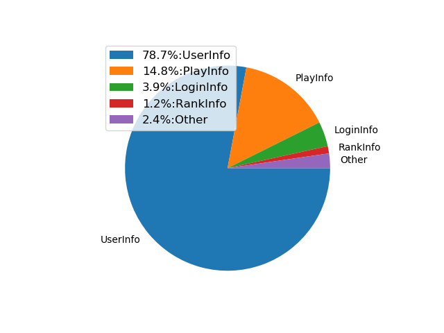
The user-type information (mainly game currency, even without 1coin and 2coin) take a major portion of the feature importances - suggesting that it is the user data that was the main contributor to abuser signals. Another main chunk was from the play data, which at first glance sounds like good information, which means some abnormalities in the game play between abusers and non-abusers were found. However, given the overwhelming dominance of game currency related information, we wonder if the model based its choices too much on game currency (which in our case was a result of our own doing, since we did label the data based on game currency).
The conclusion here is that this random forest classifier works well, but shows signs of overfitting, and we would proceed onto the hyperparameters to check what exactly the culprit could be, and how we can try to achieve a balance between the two.
Data imbalance
As reported earlier, the number of non-abusers and abusers are about 6 to 1. If there is an overwhelming amount of data regarding one class versus the other, the model tends to make biased judgements on the minority class. Many models assume that the distributions across classes are relatively equal (even though we use random forest, which performs relatively well against noise), and hence the data weight must be adjusted to compensate for this bias in decision-making. To show how this concept can be applied, we can modify the parameter called class_weight in the Random Forest Classifier model, in the code below.
rf = RandomForestClassifier(class_weight='balanced')This helps to ensure that, per datapoint of labelled abusers, the data weight is increased so that abusers can be identified more robustly. The results with a deliberately balanced class weight is shown below.
rf_train_accuracy: 0.999306802427328
rf_train_fscore: 0.9974700344241217
rf_val_accuracy: 0.9885
rf_val_fscore: 0.9585177898016067
A short adjustment in class weight imbalance led to a 0.4% increase in validation accuracy (from 98.5% to 98.9%). Hence, these are the low-hanging fruits that we can look out for when we are trying to improve a model.
Parameter tuning
The random forest model should not be left as-is when running it on our dataset. This is because during the creation of decision trees, how finely the model can divide the data or how deeply it needs to go to categorize a data should differ on a case-to-case basis. The complexity of each type of problem is different and overfitting or underfitting can occur to problems depending on their background and situation. Hence, to diagnose and solve the problems as mentioned above, parameter tuning has to be done to dictate how the model can better adjust its decision-making process.
Here is a short summary on the hyperparameters dealt with, which are:
min_samples_splitmin_samples_leafmax_depthmax_featuren_estimators

Given the current set of results, we have done a short area under a curve (AUC) analysis on tree depth, n_estimators, max_features, a more general analysis on the min_sample_leaf/min_sample_split and also potentially a change in bootstrapping. AUC tells us the ability of the model to differentiate between classes, but may be a bit difficult to explain in this article. Do take the time to read more about it here.
Our plan is to find the best hyperparameters to tune the model to get a high accuracy for our model, but using GridSearch to run the learning models for each set of variables take time, and hence it is perhaps better to see the range of which our models overfit or underfit so that the number of iterations that is used in the GridSearch model can be cut down.
An AUC analysis with a tree depth from 1 to 30 has been done to check on the accuracy (or rather, a value that balances between false positive and false negative) to check for signs of overfitting or underfitting. Hence, in the short parameter analysis we have done below, the hyperparameter is examined to check for areas of underfitting or overfitting. Tree depth, n_estimator and max feature samples do not seem like contributing factors to overfitting.

In the case analyzing tree depth, any depth more than the 10-15 range seems to cause a slight lowering in performance in the test AUC, and is a potential alert of overfitting issues. Conversely, anything less then the 10-15 range gives a lower AUC, but very low divergence with the training AUC, and hence the idea that there is an underfitting of the data up until about 10 in depth.
Hence, any range from 10-15 is generally fine, but if time permits, the factoring of the range of Tree Depths that return a high value of AUC can be considered in the Grid Search.
n_estimators generally control the number of trees built in the classification process. More trees used would generally mean a more robust model and more accurate classification - however, the tradeoffs come in the form of possible overfitting, and also slowing down of the code. From a range of 0 to 250, there shows no real signs of overfitting below 250, and an n_estimator value of over 100 gives a marginal improvement in accuracy. Hence, using n_estimators in the GridSearch would slow down the code, and the tradeoffs by taking n_estimators= 100 would not generate such an accuracy loss.

As there are only 26 features we are taking into account, it is easy to conduct an analysis on the max_features section. The maximum 26 features seem to give the highest AUC Scores for our test result, and so there should be no real issue in taking max_features as 26.

However, the tricky portions come when we are talking about min_sample_split and min_sample_leaf. These are the portions where no clear answer can be given as the whole model changes depending on the number of samples required to be at each decision tree's leaf, or decision node. A low number in min_sample_split and min_sample_leaf allows the model to differentiate between samples. A low number in min_sample_split, for example, allows the decision tree to split 2 samples into different groups, while the min_sample_leaf dictates how many samples minimum can be in each "classification."
Hence, giving the model the ability to differentiate with a small number in both variables, greatly increases the risk of overfitting - the machine tends to read too much into variable differences and splits the samples even though they are not a different population. Since the default values of min_sample_leaf is 1, and min_sample_split is 2, it is quite clear to us that, merely running a plain random forest classification caused the overfitting. Running an AUC Score based on the two variables, we can see that the models perform poorly at lower levels, hence confirming the initial hypothesis of overfitting.
However, running the variables too high would also cause the model to underfit, as seen by the drop in Training AUC as the variable numbers are increased. Hence, it would be important to test a range of min_sample_split and min_sample_leaf to check the model accuracy for test results, and balance it with underfitting. This is because these two variables seem to be the main cause of the overfitting problem in the first place.
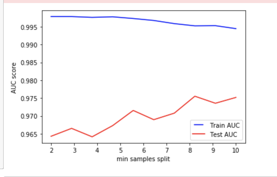
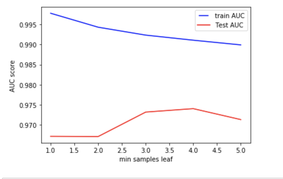
The min_sample_leaf could be possible anywhere from 2-6, while the min_sample_split could work anywhere from about 8 -10, however this is only applicable holding the rest of the parameters constant. This range we see here cannot be used for testing (i.e. change other parameters, but keep min_sample_leaf at 2-6). This is because the parameters AUC themselves will change heavily in a small tweak of other parameters.
Finally, we have the bootstrap parameter. Because the random forest is made up of many different trees, it has a few specific methods it uses to build the decision trees, and make it random - it can sample, randomly, from training datapoints, and also use a random subset of features when it splits its nodes. Bootstrapping is a parameter that impacts the way the Random Forest model draws on samples randomly, mainly if it does so with, or without replacement. While bootstrapping (sampling with replacement) is usually the ideal way to sample, because the model is able to reduce variance. However, this also means that the model will be using repeated data for training, and this runs the risk of it being overly biased. Hence, this is a tradeoff that must be taken into consideration.
Quirks and application of the tuning logic

This the same analysis for Tree Depth, but conducted with different parameters. The earlier explanation on overfitting regions has changed when we use a different set of parameters.
Left: Standard, Right: class_weight = 'balanced', min_sample_leaf= 4, min_sample_split= 3
Hence, we cannot simply conclude that for all parameters, tree depth >= 15 causes overfitting. A change in parameters (shown in the graph on the right) causes the previously seen decrease in performance for tree depth > 15 to disappear. Hence, we cannot base our observations on merely changing one parameter, while keeping other parameters constant. The results from the parameter tuning in the previous sections cannot be taken independently, as the above examples show that the areas that cause overfitting changes altogether, when the other parameters are not held constant. Therefore, the best way to find the set of parameters for the maximum performance will involve a test across a whole range of parameters, to find what the best set of parameters are. So, when we want to search for the best set of parameters, we search across a range of values for depth, estimators, and min_sample_leaf and min_sample_split.
The suggested ranges to test would be:
n_estimatorsfrom about 1 to 250max_featuresfrom 1 to maximum number, auto and sqrtmax_depthfrom 1 to 200min_samples_splitfrom 2 to 20min_samples_leaffrom 1 to 20- Bootstrap for True and False
However, while it would be the most thorough to test every single value, do keep in mind that it takes a long time to conduct a randomized search test for such a large range and number of parameters. The source code below is a simplified version to test a smaller range of parameter values, which we determined would give a higher performance.
from sklearn.model_selection import RandomizedSearchCV
# Number of trees in random forest
n_estimators = [int(x) for x in np.linspace(start = 150, stop = 250, num = 3)]
# Number of features to consider at every split
max_features = ['auto', 'sqrt']
# Maximum number of levels in tree
max_depth = [int(x) for x in np.linspace(110, 130, num = 3)]
max_depth.append(None)
# Minimum number of samples required to split a node
min_samples_split = [5, 6, 7]
# Minimum number of samples required at each leaf node
min_samples_leaf = [1, 2, 3]
# Method of selecting samples for training each tree
bootstrap = [True, False]
# Create the random grid
random_grid = {'n_estimators': n_estimators,
'max_features': max_features,
'max_depth': max_depth,
'min_samples_split': min_samples_split,
'min_samples_leaf': min_samples_leaf,
'bootstrap': bootstrap}
print(random_grid)


# Use the random grid to search for best hyperparameters
# First create the base model to tune
rf = RandomForestClassifier(class_weight= 'balanced')
# Random search of parameters, using 3 fold cross validation,
# search across 100 different combinations, and use all available cores
rf_random = RandomizedSearchCV(estimator = rf, param_distributions = random_grid, n_iter = 100, cv = 3, verbose=2, random_state=42, n_jobs = -1)
# Fit the random search model
rf_random.fit(train_X, train_y)
The resultant best model is as follows:
{'n_estimators': 200, 'min_samples_split': 7, 'min_samples_leaf': 1, 'max_features': 'sqrt', 'max_depth': 110, 'bootstrap': False}We then re-run the model using the above set-up and we get the new results as follows.
rf_train_accuracy: 0.9998181776858565
rf_train_fscore: 0.9993378031619898
rf_val_accuracy: 0.9917272727272727
rf_val_fscore: 0.9706451612903225
A good improvement from 0.9885 accuracy to 0.9917 accuracy in the validation set.
The numbers are as follows:
| Training data | Prediction | ||
|---|---|---|---|
| Abuser | Non-abuser | ||
| Labels | Abuser | 3,009 (TP) | 0 (FN) |
| Non-abuser | 16 (FP) | 18,809 (TN) | |
| Training data | Prediction | ||
|---|---|---|---|
| Abuser | Non-abuser | ||
| Labels | Abuser | 12,073 (TP) | 83 (FN) |
| Non-abuser | 99 (FP) | 75,909 (TN) | |
In general, there has been a tradeoff between training data accuracy and validation data accuracy. While there has been less ability to generalize within the training data set, the false detection statistics in the validation data set has improved. It is more important for the model to be able to generalize on other data sets, rather than just on its own data set.
General thoughts & evaluation
There seems to be good potential for random forest models to be used in game currency cheating detection. While there are still quite a number of false detections within our used data sets, it is not something we can avoid without more time to tune and re-run the algorithms. A wider range of parameters has to be tested, and more time has to be invested in the research of the best set of parameters to use. A larger data set can also be used to improve accuracy.
That said, we also need to be wary of false detections. A false positive may not necessary mean that the abuser is not a cheater - that is, the abuser could be using a 32X multiplier cheat, but since the abuser is still in low levels, they do not have abnormally high game currencies with respect to the population, but they would have abnormally high values when compared to players at the same level. Hence, perhaps one improvement that would be looked at is the outlier detection per level for these game currencies or game scores. As mentioned earlier, this is a rule-based algorithm, a similar concept to what some other tech giants use for their game abuse detection (creating rules, then adjusting their model's rules to detect those who deliberately go around it initially). There is bound to be cheaters who are just skirting the rules made, but still pass the algorithm's judgement.
Overall, this was quite a fun experience, but the ML journey does not end here. Our goal is to succeed in the automation and accuracy of our banning process, so that we can give the best gaming experience to our users by putting everyone on the common ground.
Special thanks to Myeongjae, Aiko, and Seongun, all of whom helped out in the refinement of the approach to the problem, and the content of this article.