
Greetings from Fukuoka! My name is Yanjin Li, but people call me YJ ?. I'm a data scientist from LINE Fukuoka’s Data Labs Team. I have been working with media data as part of my daily work, and in this post I want to talk about how we as data scientists are facing model trust challenges with media data. ??️
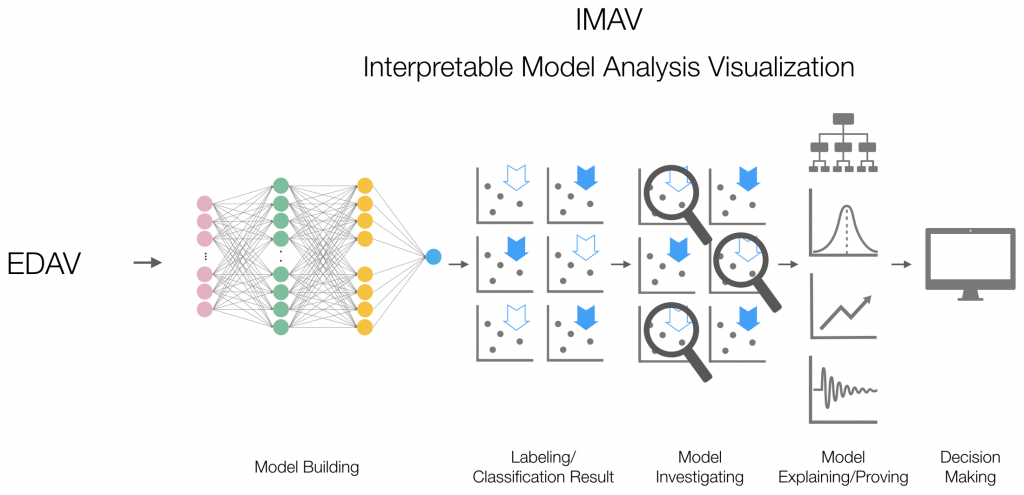
1. Overview
In order to analyze massive datasets, more and more sophisticated machine learning models are being invented. However, there is a trade-off between complexity and accuracy. Without sufficient interpretability, models are generally not trustworthy. I will talk about how to win this model trust challenge without harming accuracy through the following example. All the source code can be found here Github source code link.
A majority of hands-on project posts usually emphasize Exploratory Data Analysis and Visualization (EDAV) and model training. However, in this post I want to go more in-depth on the challenges in interpreting the models by multiple post-model-training analysis techniques. As a Data Scientist, I sometimes face the constraints of relying only on measuring accuracy on some held out data or cross-validation. This method is acceptable but also has some pitfalls, for example training classifiers that were run on imbalanced or leaked data.
In this post, I will conduct the four steps shown in the following flow-chart, after which we will be able to choose between competing models as well as detect and improve untrustworthy ones and get insights into them. The example will show how a model is trustworthy not only on the training dataset but also in real-world examples. After seeing the explanations, you will start to have a solid insight into what makes a model trustworthy and why.
Now, let's start to work on an example using IMDB data.
1.1 Introduction of Packages
I will introduce a few recently-released packages in the following section.
keras: a model-level library, providing high-level building blocks for developing deep-learning models.limeshort for Local Interpretable Model-agnostic Explanations: an explanatory package for black box complex classifiers. Instead of providing a complete model, the package shows some approximations that can describe/represent how the model is actually behaving.corrr: a tidy correlation analysis package.yardstick: a tidy model performance measuring package.
1.2 Environment Initialization
# data processing
library(tidyr)
library(dplyr)
library(knitr)
library(kableExtra)
# data visualizations
library(corrplot)
library(ggplot2)
library(forcats)
library(corrr)
library(yardstick)
# model training
library(keras)
library(lime)
library(recipes)
We also need to build a few helper functions, which will be used during the data processing and model training procedures:
# vectorize sequences
vectorizeSequences <- function(sequences) {
  results <- matrix(0, nrow = length(sequences), ncol = word.dim)
  for (i in 1:length(sequences))
    results[i, sequences[[i]]] <- 1
  results
}

# transform from index
transformNameFromIndex <- function(input.data){
  # change the column names by index
  names(input.data) <- plyr::mapvalues(names(input.data),
                                       # change from index
                                       from = lst.data$index$index,
                                       # to real words
                                       to = lst.data$index$word)
  return(input.data)
}

# define our own predict_model() to reformat binary encoding
predict_model.keras.models.Sequential <- function (x, newdata, type, ...) {
  pred <- predict_proba (object = x, x = as.matrix(newdata))
  data.frame (Positive = pred, Negative = 1 - pred) }
2. Data Preparation
First all of, I will define a variable which describes the maximum number of words we want to include. Additionally, words are ranked by how often they occur (in the training set) and only the most frequent words are kept.
# define the number of words/dimensions
word.dim <- 2000
skip.dim <- 20
2.1 Data Source
I chose to use a dataset of 25,000 movie reviews from IMDB, labeled by binary sentiment (either negative or positive reviews). Each review has been encoded as a bag of words format, with word indexes (integers). Let's also look at the index list first:
# create a data container
lst.data <- c()
# extract the word index
lst.data$index <- unlist(dataset_imdb_word_index()) %>%
  # cast from list to a dataframe
  as.data.frame() %>%
  # define column names
  tibble::rownames_to_column(., "word") %>%
  rename(index = ".") %>%
  mutate(index = paste0("V", index))

# show the data in a tidy way
lst.data$index[1:6,] %>% kable() %>%
  kable_styling()
| word | index |
|---|---|
| fawn | V34701 |
| tsukino | V52006 |
| nunnery | V52007 |
| sonja | V16816 |
| gag | V3285 |
| woods | V1408 |
For convenience, words are indexed by overall term frequency. For example, a word with index 3 represents the 3rd most frequently used term in the whole training data. Therefore, by setting a word.dim equal to 2,000 and skip.dim equal to 20, we can consider the top 2,000 most common words while eliminating the top 20 amongst those. Let's first extract the raw data:
# choose no more than 1000 words to include
lst.data$raw <- dataset_imdb(num_words = word.dim)
# lst.data$raw <- dataset_imdb(num_words = word.dim, skip_top = skip.dim)
2.2 Data Processing
Right now, the lst.data$raw list includes multiple tables/vectors:
lst.data$raw$train$xlst.data$raw$train$ylst.data$raw$test$xlst.data$raw$test$y
Now vectorizing and restructuring the above list with the helper functions defined in the previous code section, we get:
# vectorize the raw training dataset
lst.data$train <- vectorizeSequences(lst.data$raw$train$x) %>%
  as.data.frame() %>%
  # column combined with y values
  cbind(., data.frame(predicting_value_y = as.numeric(lst.data$raw$train$y)))

# map name from the index table
lst.data$train <- transformNameFromIndex(lst.data$train)

# view train data
lst.data$train[1:10, 1:5] %>% kable() %>%
kable_styling()| the | and | a | of | to | is | br | in | it | i |
|---|---|---|---|---|---|---|---|---|---|
| 1 | 1 | 0 | 1 | 1 | 1 | 1 | 1 | 1 | 0 |
| 1 | 1 | 0 | 1 | 1 | 1 | 1 | 1 | 1 | 0 |
| 1 | 1 | 0 | 1 | 0 | 1 | 1 | 1 | 1 | 0 |
| 1 | 1 | 0 | 1 | 1 | 1 | 1 | 1 | 1 | 1 |
| 1 | 1 | 0 | 1 | 1 | 1 | 1 | 1 | 0 | 1 |
Apply the same technique to the test dataset:
# vectorize the raw test dataset
lst.data$test <- vectorizeSequences(lst.data$raw$test$x) %>%
  as.data.frame() %>%
  # column combined with y values
  cbind(., data.frame(predicting_value_y = as.numeric(lst.data$raw$test$y)))

# map name from the index table
lst.data$test <- transformNameFromIndex(lst.data$test)
Now, I will start to split data into X matrix and y vector:
# extract x in training set
lst.data$train.x <- lst.data$train %>%
  select (-predicting_value_y)
# replace NA with 0
lst.data$train.x[is.na(lst.data$train.x)] <- 0

# extract x in test set
lst.data$test.x <- lst.data$test %>%
  select (-predicting_value_y)
# replace NA with 0
lst.data$test.x[is.na(lst.data$test.x)] <- 0
Extract the dependent variable y in a vector format:
# Extract Y vectors
lst.data$train.y <- as.vector(lst.data$train$predicting_value_y)
lst.data$test.y  <- as.vector(lst.data$test$predicting_value_y)
3. Building Network
In this project, I chose a relatively shallow neural network with 1 input layer, 3 hidden layers, and 1 output layer. This model serves as a jumping-off point and an experimental step for more complex algorithms.
3.1 Build Multi-Layer Perceptron (MLP)
Prior to running an algorithm to classify the binary reviews, we will need to first create building blocks for our NN framework. As you can see due to the volume of our input data, we have 32,305 trainable parameters.
model_keras <- keras_model_sequential()

model_keras %>%
  # (1) 1st Hidden Layer-------------------------------------------------
layer_dense (units              = 16, #=> Num Of Nodes
             kernel_initializer = "uniform",
             activation         = "relu",
             input_shape        = ncol(lst.data$train.x)) %>%
  ##layer_dropout (rate = 0.1) %>%  #=> Dropout Below 10%: Prevent overfitting
  # (2) 2nd Hidden Layer-------------------------------------------------
layer_dense (units              = 16,
             kernel_initializer = "uniform",
             activation         = "relu") %>%
  ##layer_dropout (rate = 0.1) %>%
  # (3) Output Layer-----------------------------------------------------
layer_dense (units              = 1, #=> Binary/Multi?=>That Number
             kernel_initializer = "uniform",
             activation         = "sigmoid") %>% #=> Common for Binary
  # (4) Compile Model-----------------------------------------------------
compile (optimizer = 'adam', #=> Most Popular for Optimization Algo.
         loss      = 'binary_crossentropy', #=> Binary Classification
         metrics   = c('accuracy') ) #=> Train/Test Evaluation

# Check model structure
model_keras
## Model
## ___________________________________________________________________________
## Layer (type) Output Shape Param #
## ===========================================================================
## dense_1 (Dense) (None, 16) 32016
## ___________________________________________________________________________
## dense_2 (Dense) (None, 16) 272
## ___________________________________________________________________________
## dense_3 (Dense) (None, 1) 17
## ===========================================================================
## Total params: 32,305
## Trainable params: 32,305
## Non-trainable params: 0
## ___________________________________________________________________________
Fit keras_model to the training dataset,
history <- model_keras %>% fit(
object = .,
x = as.matrix(lst.data$train.x),
y = lst.data$train.y,
epochs = 20,
batch_size = 512,
validation_split = 0.30
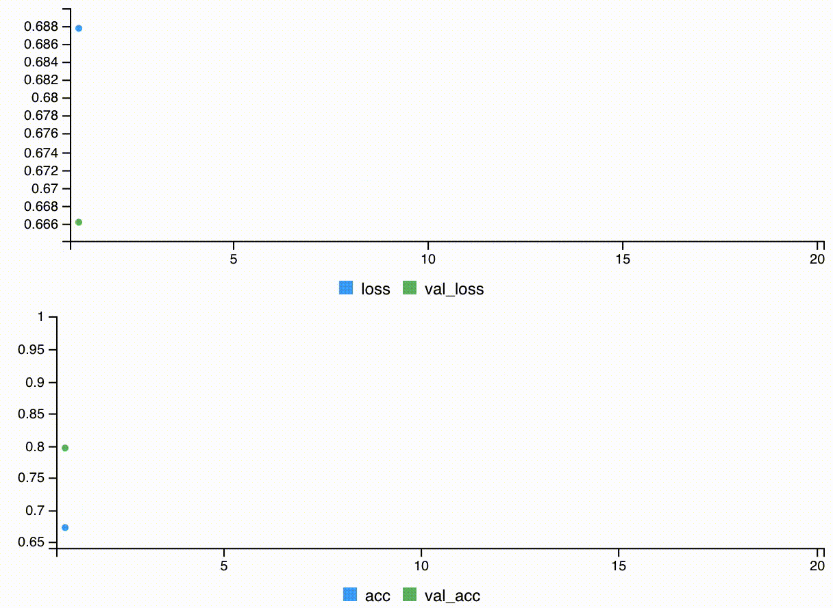
)Visualize the training history,
4 Interpretable Model Analysis and Validation
4.1 Model Validations
Now, we can run our model on the test set to validate the model performance. Here, I have used two type of generators. predict_classes is used for generating class values as a matrix of binary ones and zeros. predict_proba is used for generating class' corresponding probabilities as a numeric matrix indicating the probability of being a class (the probabilities computed based on majority voting results).
# generate the class predictions
yhat_keras_class_vec <- predict_classes(object = model_keras,
                                        x = as.matrix(lst.data$test.x)) %>%
  as.vector()

# generate the class probabilities predictions
yhat_keras_prob_vec <- predict_proba(object = model_keras,
                                     x = as.matrix(lst.data$test.x)) %>%
  as.vector()
Before running model validations, we will need to create a data frame to store:
truth: the actual review valuesestimate: predicted values as factorsclass probability: the probability of being 1 class (positive reviews)
# re-fresh evironment
options(scipen = 999)
options (yardstick.event_first = FALSE)

estimates_keras_tbl <- tibble(
  # define the truth
  truth      = as.factor(lst.data$test.y) %>%
    # factorize 1 and 0
    fct_recode(Positive = "1", Negative = "0"),
  # join estimate
  estimate   = as.factor(yhat_keras_class_vec) %>%
    fct_recode(Positive = "1", Negative = "0"),
  # join probabilities of estimation
  class_prob = yhat_keras_prob_vec )

# visualize the table
estimates_keras_tbl[1:5, ] %>%
  kable() %>%
kable_styling()| truth | estimate | class_prob |
|---|---|---|
| Negative | Negative | 0.0445649 |
| Positive | Positive | 0.9995100 |
| Positive | Negative | 0.1141590 |
| Negative | Positive | 0.8948936 |
| Positive | Positive | 0.8953462 |
4.1.1 Accuracy
As you can see, we are getting roughly ~85.70% accuracy. However, under some circumstances, this high accuracy might be caused by imbalanced data. Thus, as a next step, let's investigate the model by looking at the confusion matrix.
estimates_keras_tbl %>%
  metrics(truth, estimate)

# 0.85696
4.1.2 Confusion Matrix
In order to describe the performance of our classifier on the test dataset, we will deliver a confusion matrix. In our example, we will focus specifically on preventing misclassifications where a user’s review is actually negative, but we predicted it as positive. Our confusion matrix is,
estimates_keras_tbl %>%
conf_mat(truth, estimate)| Prediction/Truth | Negative | Positive |
|---|---|---|
| Negative | 10639(85.11%) | 1715(13.72%) |
| Positive | 1861(14.89%) | 10785(86.28%) |
4.1.3 AUC
Also, we can conduct a Receiver Operating Characteristic (ROC) Area Under the Curve (AUC) measurement in order to compare our model with a random guessing method, which has AUC = 0.50. AUC using normalized units can deliver the probability that a classifier will rank a randomly chosen positive instance higher than a randomly chosen negative one.
estimates_keras_tbl %>%
  roc_auc(truth, class_prob)
  # 0.9299374
4.1.4 Precision and Recall
By looking at precision and recall, we can understand the model relevancy. Precision is the fraction of relevant instances among the retrieved ones, while recall is the fraction of relevant instances that have been retrieved over the total amount of relevant instances.
tibble (
  precision = estimates_keras_tbl %>% precision(truth, estimate),
recall = estimates_keras_tbl %>% recall(truth, estimate))| precision | recall |
|---|---|
| 0.8528 | 0.8628 |
4.1.5 F1-Score
F1 score considers both the precision and the recall of the test to compute the score. The closer to 1 the better.
estimates_keras_tbl %>%
  f_meas(truth, estimate, beta = 1)
 #  0.8577905
Based on the above observations of model performance, we can draw a preliminary conclusion that our model performs well in terms of predictions. However, from a business perspective, these metrics are less straightforward and less relevant to the model itself than its final performance. Therefore, as a next step, I will start to work on how to interpret our model by 'seeing' the complex black box model using LIME.
4.2 Model Interpretation
In this section, I will talk about how to interpret a complex and accurate model using multiple packages. First of all, we need to let the LIME package know the type of model we are investigating, i.e. classification.
class(model_keras)

# define the type of model passed through LIME
model_type.keras.models.Sequential <- function(x, ...) {
  "classification"}
## [1] "keras.engine.sequential.Sequential"
## [2] "keras.engine.training.Model"
## [3] "keras.engine.network.Network"
## [4] "keras.engine.base_layer.Layer"
## [5] "python.builtin.object"
4.2.1 Initial Setups
Then, we will start to use the helper function we defined previously, lime::predict_model(), for our keras_model to run the local model-performance-agnostic functions,
# visualize the output of our defined functions
predict_model(x = model_keras,
               newdata = lst.data$test.x,
               type    = 'raw') %>%
tibble::as_tibble()| Response |
|---|
| 0.0445648878812789917 |
| 0.9995100498199462891 |
| 0.1141589507460594177 |
| 0.8948936462402343750 |
| 0.8953462243080139160 |
Now, we can start conducting the explanation process by passing the training set into the lime::lime function, which is a factory function that returns a new function that can be used to explain the predictions made by black box models.
explainer <- lime::lime(
  x              = lst.data$train.x,
  model          = model_keras,
  bin_continuous = FALSE)
# view the explainer
# explainer
Then, we can use the lime::explain to return the explanations of our classification model.
explanation <- lime::explain(
    as.data.frame(lst.data$test.x)[1:6, ], # Just to show first 6 examples
    explainer    = explainer,
    n_labels     = 1, # explaining a `single class`(Review)
    n_features   = 10, # returns top 10 features critical to each case
    kernel_width = 0.5) # allows us to increase model_r2 value by shrinking the localized evaluation.
4.2.2 Feature Importance
In the following 6 example feature importance plots, Label 1 represents Negative reviews (binary code 0), and Label 2 represents Positive reviews (binary code 1). The green bar represents how "supportive" a factor is, and the red bar represents how "uncontradicted" a factor is. For example, in Case #1, the words "hope" and "sure" support predictive results while words like "supporting" and "drugs" undermine predictive results. Based on the majority vote by factors, the predictive results will be delivered. As you can see, most of the Negative-review-oriented words do make sense, such as "hope". However, the word "death" and "zombie" are misleading. This is one type of pitfall I mentioned earlier in this post.
plot_features (explanation) +
  labs (title = " Feature Importance Visualization",
        subtitle = "Hold Out (Test) Set, First 10 Cases Shown")
4.2.3 Feature Heatmap
plot_explanations(explanation) +
  labs(title = "Feature Importance Heatmap",
        subtitle = "Hold Out (Test) Set, First 10 Cases Shown")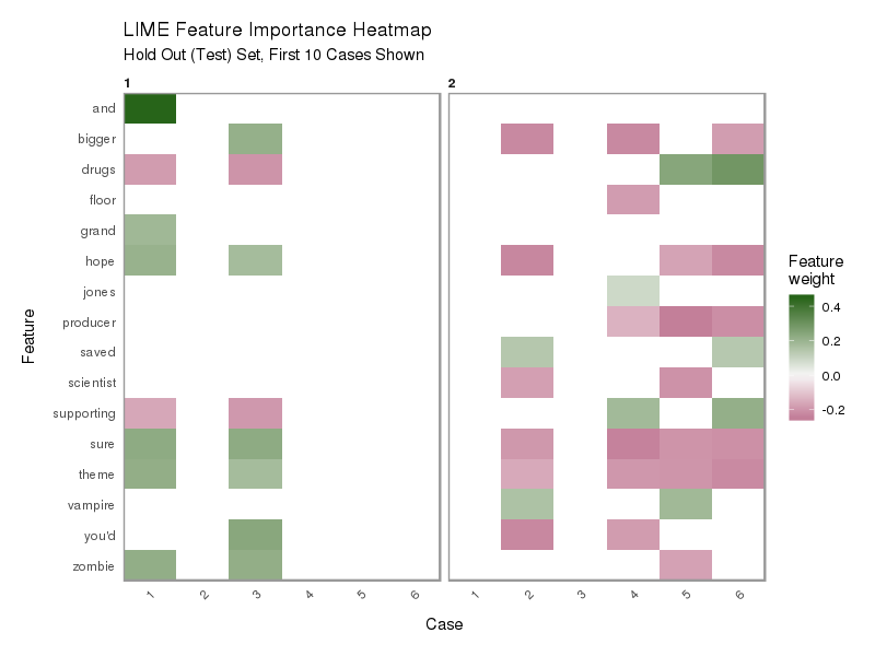
4.2.4 Feature Correlations
Now let's compute the feature correlations to the binary reviews.
# conduct correlation analysis
corrr_analysis <- lst.data$train.x %>%
    mutate (Score = lst.data$train.y) %>%
    correlate () %>%
    focus (Score) %>%
    rename (feature = rowname) %>%
    arrange (abs(Score)) %>%
    mutate (feature = as_factor(feature))

# keep the top 50 variables ranked by scores
corrr_analysis_viz <- corrr_analysis %>%
  top_n(., 50, Score) %>%
  # keep the bottom 50 variables ranked by scores
  rbind(., corrr_analysis %>%
          top_n(., -50, Score) )

# view the correlation values
corrr_analysis_viz[1:5,]| feature | Score |
|---|---|
| itself | 0.07242915 |
| romantic | 0.07244069 |
| witty | 0.07287877 |
| need | 0.07311425 |
| course | 0.07365957 |
Finally, let's visualize the correlation by ranks to distinguish which features are more relevant to binary reviews than others.
# visualize the result
corrr_analysis_viz %>%
  ggplot(aes(x = Score, y = fct_reorder(feature, desc(Score)))) +
  geom_point() +
  # Positive Correlations - Contribute to Polarity--------------------------------------------
geom_segment(aes(xend = 0, yend = feature),
             color = line_colors[["green"]],
             data = corrr_analysis_viz %>% filter(Score > 0)) +
  geom_point(color = line_colors[["green"]],
             data = corrr_analysis_viz %>% filter(Score > 0)) +
  # Negative Correlations - Prevent Polarity--------------------------------------------------
geom_segment(aes(xend = 0, yend = feature),
             color = line_colors[["red"]],
             data = corrr_analysis_viz %>% filter(Score < 0)) +
  geom_point(color = line_colors[["red"]],
             data = corrr_analysis_viz %>% filter(Score < 0)) +
  # Vertical lines-------------------------------------------------------------------------
geom_vline(xintercept = 0, color = "#132F5E", size = 0.5, linetype = 2) +
  geom_vline(xintercept = -0.25, color = "#132F5E", size = 0.5, linetype = 2) +
  geom_vline(xintercept = 0.25, color = "#132F5E", size = 0.5, linetype = 2) +
  # Aesthetics-----------------------------------------------------------------------------
theme_bw() +
  labs(title = "Feature Correlation Rank",
       subtitle = "Positive Correlations vs. Negative Correlations",
       y = "Feature Correlation")
On one hand, the negative (red) variables share more similar wording. For example, "do", "hope", "perhaps", "even", "little", "absolutely", "since", "which", and "imagine" are all words used when people made improvement related comments, such as "I hope the movie can have more details which perhaps can make the entire movie make more sense". Additionally, words such as "movie's", "entire", "films", "rest", "director" indicated that the topic of those negative comments was movie quality-centric. On the other hand, you may ask why positive comments shared relatively less obvious wording style in common. One hypothesis is that when leaving a comment to compliment a movie, the words used can be very specific to the movie being commented on. Therefore, the indicative words towards positive reviews are like step-words.
In short, the trustworthiness of our model is proved not only by accuracy-measuring metrics, but also by interpretable charts. However, when the movie theme involves "zombie", "death" or "drug", the prediction needs more manual inspection from us data scientists.
5. Summary
In this post, I introduced a methodology for interpreting data post-modeling, which I’m calling Interpretable Model Analysis and Visualization. The method is focused on how to overcome model trust challenges with interpretable metrics and charts. Hope you enjoyed it!
6. Acknowledgments
I would like to thank my LINE colleagues, Horikawa-san, Kengo-san, Oho-san, Parth-san and Yan-san, who provided insight and expertise that greatly assisted the blog.
The next post (2018/12/14) is “簡単なトライ” from Uemura-san. お楽しみに! ??